Blog - Purdue-P - An Exploration into Probabilistic Spin Logic (p-bits)

I've heard of Quantum Computing, now what's
Probabilistic Computing?

10/04/19 - Lakshmi A. Ghantasala

With Moore’s law coming to an end within the next decade, beyond CMOS technology is being studied with greater intent than ever before. Among the most popular of these alternative computing methods is quantum computing. Google’s recent claim of quantum supremacy has put this computing paradigm in the spotlight as the future of computing. While quantum may well be the future, this technology is still decades from maturing to a scale that can rival today’s CMOS technology. How then can we continue to progress over the next 20 or 30 years?

Probabilistic spin logic is a computing paradigm that may just have the necessary qualities to fit this requirement. A probabilistic computer was even hinted at by Feynman in his famous “Simulating Physics with Computers” paper back in 1982; he talks about how a probabilistic nature could be simulated simply by “a “computer that itself is probabilistic”. Fast forward to 2019, and an 8-bit probabilistic computer that can factorize integers has been demonstrated, which you can read about here. To be clear, we could model a probabilistic computer with existing CMOS technology for years, but a real probabilistic computer had yet to be built.

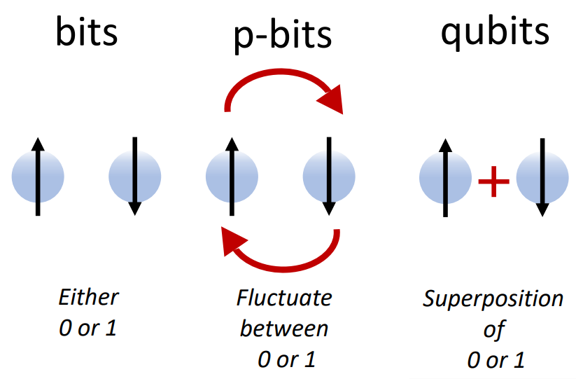
A couple of key differences from quantum computers makes this new probabilistic paradigm more appealing for the immediate future. One, p-bits can operate at room temperature, while qubits require extensive engineering to keep temperatures close to sub-zero. Second, p-bits are entirely classical by nature. There are no decoherence issues that limit distance or strength of connections. This allows p-computers to follow the same rules that affect transistor technology. Luckily, we have a half-century of experience already in place. Probabilistic spin logic is a name given to the study of these networks of p-bits, and bringing them together to build p-computers.

With the rest of this post, I hope to explain some of the driving principles behind Probabilistic Spin Logic. This is by no means a comprehensive guide; rather it should help give an idea of how p-bits solve problems.

The p-bit is at the heart of a p-computer

A p-bit can be broken down into two behavioural components. First, the neuron’s behaviour, and second, the input bias. The neuron’s behaviour can be summarized by the following equation.

mi=sgn[tanh(Ii)−r]

A p-bit outputs the sign of the input minus a random number over the range of that input. Simply put, if the bias into a p-bit is high, then it will likely occupy a state of 1. If the input bias is small, it will likely occupy a state of -1. At a 50% input bias, the p-bit occupies a random state at any time, switching rapidly between + and - 1. The second component is the input to the p-bit. This input is generated according to the following equation.

Ii = ∑jWijmj

The input to p-bit i is simply the sum of all the weights connected to p-bit i multiplied by their respective source p-bits. These two simple rules govern the behaviour of a probabilistic computer.

Putting Problems on a Probabilistic Computer

In order to take advantage of a probabilistic computer, problems must be phrased in a way that the p-computer understands. The way we phrase these problems is in the form of a set of weights. Weights can be intelligently designed to capture the constraints of some problem; the solution to the problem we want to solve is hidden in those weights. The p-bits of the p-computer, when connected to each other by that set of weights, will fluctuate until they satisfy those constraints the best they can. At that stage, the p-bits have reached some low energy state, and they tend to settle in. Though they will continue to fluctuate, as a whole, they won’t fluctuate too far from that low energy state. We can encourage the p-bits to find the lowest energy state rather than some sub-optimal low state by starting the network at a high temperature, and slowly cooling the network until the p-bits settle in to their preferred states. There exist many annealing patterns or schedules we can follow to enhance the p-computer’s ability to find the lowest energy ground state.

Multi-p-bit gates

*p-bits emulating a multiply (and) gate.*

Probabilistic algorithms have been developed that allow us to model logic gates on a p-computer. For example, let’s imagine a multiply gate. This is a 3-p-bit gate in which p-bit A multiplies with p-bit B to get p-bit C. Immediately, the states which satisfy this gate are clear to us. For instance, 0 and 0 multiply to get 0.Likewise, 0 x 1 = 0, 1 x 0 = 0, and 1 x 1 = 1. There are 4 states that these p-bits can occupy that hold true to a multiply gate. Left to its own devices, a 3-p-bit network encoded with “multiply gate weights” will probabilistically occupy these 4 states over all the others. Try this problem out in the Purdue-P web simulator!

A Simple Guide to J and h

9/25/19 - Lakshmi A. Ghantasala

J and h are all you really need to describe some unique p-circuit. They encode the constraints of the problem, and will lead a p-circuit to a ground state that solves that problem.

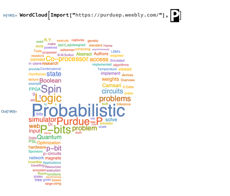
Purdue-P Word Cloud

7/30/19 - Kerem Camsari

The contents of https://www.purdue.edu/p-bit were pulled and a word cloud was made in mathematica. The following line of code made this possible. The attached version of the p is a specialized version, where names and pronouns were manually removed.